Break end-to-end latency into network, CPU, database, serialization and queueing components, measure each with the right tool, estimate them with rules of thumb, find the dominant component, and pick the tactic that addresses it
Covers
Network · CPU · Database · Serialization · Queueing
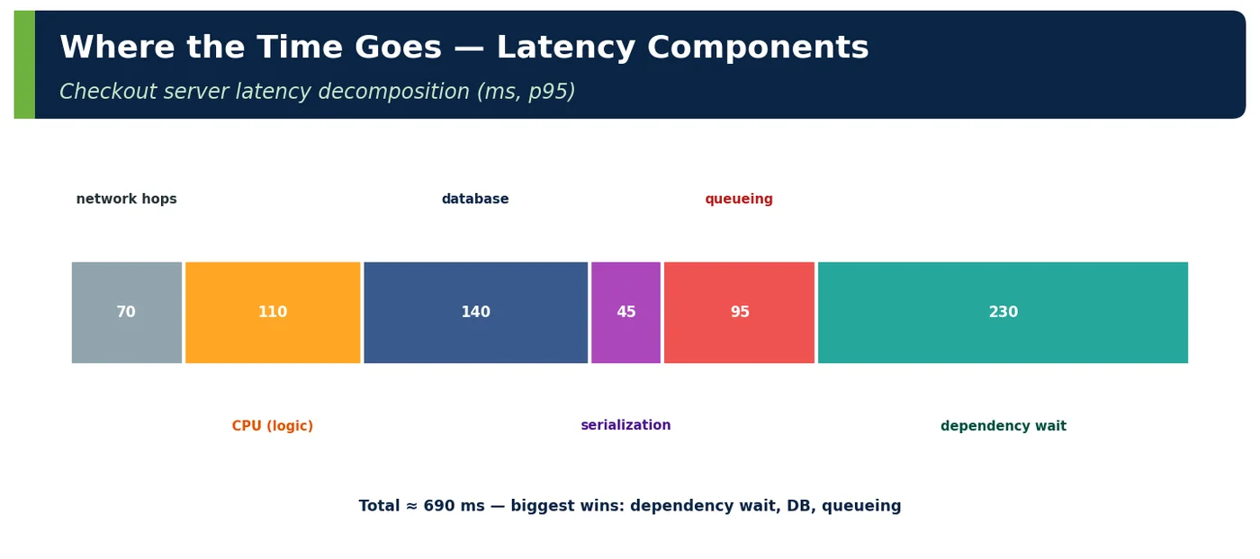
End-to-end latency is the sum of time spent in five kinds of activity on the critical path. Optimising without decomposing is guesswork.
Figure 1 — Where the time goes — latency components
Component
What consumes time
Typical range (per hop)
Network
Propagation, RTTs, TLS handshakes, bandwidth
0.3 ms (same AZ) … 80 ms (4G)
CPU
Business logic, framework overhead, GC, crypto
0.1 … 200 ms
Database
Parsing, planning, I/O, locks, round trips
1 … 100+ ms
Serialization
Encoding/decoding JSON, protobuf, compression
10 µs … 5 ms
Queueing
Waiting for threads, connections, locks, partitions
0 … unbounded
Table 1 — Five components
2Why It Exists
A request crosses many components, each with its own cost and failure modes. Without decomposition teams rewrite code (CPU) when the time is in a sequential network chain, or scale pods when the time is in a database lock.
4How It Works Internally — Decomposing with Traces
Step
Tool
Output
1
OpenTelemetry Java agent on all services
Spans per hop
2
Group spans by type (HTTP client, DB, messaging)
Time per component
3
Identify critical path (sequential spans)
What actually matters
4
Add JFR profile for CPU-heavy spans
Hot methods
5
Compare with pool/queue metrics
Wait vs work
6
Build latency budget table
Owner per component
Table 8 — Decomposition method
Span (checkout p95)
Duration
Component
On critical path?
HTTP server span
690 ms
Total
—
gRPC pricing
110 ms
Network + CPU
Yes (parallel with inventory 90 ms)
JDBC (6 statements)
140 ms
Database
Yes
HTTP gateway
230 ms
Network + dependency
Yes
JSON encode/decode
45 ms
Serialization
Yes
Waiting for pool/thread
95 ms
Queueing
Yes
Logic
70 ms
CPU
Yes
Table 9 — Trace-based breakdown
4ADeep Dive — Service Time vs Waiting Time
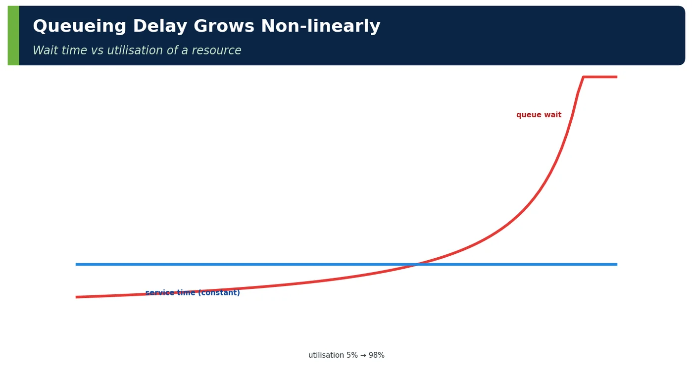
Every component has service time (doing work) and waiting time (queued). Waiting depends on utilisation: W_queue ≈ S × ρ/(1−ρ) for a simple queue. That means you can reduce latency without making anything faster — by lowering utilisation (more capacity) or smoothing bursts.
Utilisation
Service 100 ms → total latency
50%
≈ 200 ms
70%
≈ 330 ms
90%
≈ 1,000 ms
Table 10 — Same code, different latency
5APIs / Features / Syntax
BASH
# Profile a running checkout pod for 60 s (JDK Flight Recorder, Java 25)jcmd 1 JFR.start name=perf duration=60s settings=profile filename=/tmp/checkout.jfrjfr print --events jdk.ExecutionSample /tmp/checkout.jfr | head -50jfr summary /tmp/checkout.jfr # GC pauses, allocation, lock contention
// Protobuf for internal gRPC calls instead of JSON (serialization component)PriceQuote quote = pricingStub.withDeadlineAfter(150, TimeUnit.MILLISECONDS) .quote(QuoteRequest.newBuilder().addAllSkus(cart.skus()).build());
Component
Primary tool
Network
Traces, VPC flow logs, RUM
CPU
JFR, async-profiler
Database
Performance Insights, pg_stat_statements, EXPLAIN
Serialization
JFR allocation + CPU samples, JMH
Queueing
Pool metrics, executor metrics, consumer lag
Table 11 — Tools per component
6Practical Examples
6.1 ShopNow checkout: largest slice first
Component
Before
Change
After
Dependency wait (gateway)
230 ms
Connection pool 20 → 40, keep-alive
160 ms
Queueing
95 ms
Pool tuning, 70% CPU target
20 ms
Database
140 ms
6 → 2 round trips (batching)
95 ms
Serialization
45 ms
Smaller DTO, protobuf to pricing
20 ms
Table 12 — Result: p95 690 → 480 ms
6.2 GC spikes
Checkout p99 spiked every 20 s. GC logs showed 180 ms G1 pauses from 2.4 MB allocation per request. Reducing allocation (reusing buffers, records instead of maps) and switching to generational ZGC cut pauses to < 1 ms.
6.3 Cross-AZ chattiness
A pricing call made 14 cache lookups to a Valkey node in another AZ (~1 ms each). Batching into one MGET removed 13 ms from p50.
6.4 Worked example — network arithmetic
Pattern
RTTs
Latency at 1 ms RTT
10 sequential calls
10
10 ms + work
10 parallel calls
1 (max)
~1 ms + slowest work
1 batched call
1
~1 ms + batch work
Table 13 — Round trips dominate at scale
6.5 Worked example — payload diet
Change
Payload
p95 transfer on 4G
Full product entity
900 KB
1.4 s
DTO with needed fields
180 KB
300 ms
+ brotli
40 KB
70 ms
Table 14 — Serialization + network
6.6 Worked example — component table for an interview
Component
How I'd find it
Tactic
Network
Trace spans per hop
Fewer hops, parallel, keep-alive
CPU
Flame graph
Algorithm, allocation
DB
Performance Insights
Index, batch
Serialization
Profile encode/decode
Smaller DTO, binary format
Queueing
Pool pending metrics
Headroom, pool sizing
Table 15 — Structured answer
Figure 7 — Component → main tactics
6.7 Worked example — estimating latency before building
Design: product page API
Estimate
Client ↔ CloudFront (Mumbai, 4G)
60 ms RTT
CloudFront → ALB (cache miss)
5 ms
Service CPU (JSON 30 KB)
12 ms
Valkey lookup (same AZ, 1 call)
1 ms
Aurora reader (cache miss, indexed)
4 ms
Serialization
2 ms
Server latency
≈ 20 ms (hit) / 25 ms (miss)
Response time (4G, warm connection)
≈ 90–120 ms
Table 16 — Back-of-envelope before writing code
6.8 Worked example — lock queueing on a hot row
Observation
Value
Inventory update p99
1.8 s at flash sale
DB CPU
35% (not busy)
Lock wait (Performance Insights)
92% of DB time
Fix
Reserve via conditional UPDATE per SKU + sharded counters for the hottest SKU
Result
p99 45 ms
Table 17 — Queueing hidden as "database latency"
6.9 Worked example — the same request in three regions
Client location
RTT to ap-south-1
Response time p95
Mumbai
12 ms
240 ms
Kolkata
35 ms
300 ms
Singapore customers
60 ms
420 ms
Table 18 — Distance is a latency component you cannot optimise away — only move closer
7Common Problems & Mistakes
Mistake
Fix
Optimising CPU when network dominates
Trace first
Ignoring waiting time
Pool/queue metrics
Chatty services across AZs
Batch, co-locate
Large payloads to mobile
DTOs, compression
GC ignored
Allocation profiling, modern collectors
Treating DB as one number
Break into pool, RTT, execution, locks
Table 19 — Mistakes and fixes
8Performance & Production Considerations
Consideration
Practice
Continuous profiling
Low-overhead JFR in production
Trace sampling
Tail-based sampling keeps slow traces
Component dashboards
DB time, dependency time, queue time per service
Regression detection
JMH for serialization hot paths
Table 20 — Operating component visibility
Component visibility has to be permanent, because latency regressions usually arrive with a dependency upgrade, data growth or a traffic shift rather than with an obvious code change. Run JFR continuously in production with the default settings, which cost around 1% overhead, so a profile already exists when p99 moves. Use tail-based sampling in the OpenTelemetry Collector so the slowest and failed traces are always kept, rather than a random 1% that rarely contains the outliers you need. Each service dashboard should split time into database, dependency, queue and own-CPU time, so a shift between components is visible at a glance. Finally, guard serialization and other hot paths with JMH benchmarks in CI, and run a load test against the latency budget before every peak event.
9Architecture & Design Considerations
Guideline
Detail
Minimise sequential network hops
Coarser APIs, parallel fan-out
Keep data close to compute
Caches, same-AZ reads
Choose efficient internal formats
gRPC/protobuf between services
Design for low utilisation of shared resources
Queueing is the silent component
Table 21 — Design guidance
10Interview Questions & Answers
Q1BasicConcept
Name the five latency components.
The five components are network, CPU, database, serialization and queueing. Network time covers propagation, round trips, TCP and TLS handshakes and bandwidth. CPU time is business logic, framework overhead, garbage collection and crypto. Database time includes pool wait, query parsing and planning, execution and I/O, lock waits and result transfer. Serialization is encoding and decoding JSON or protobuf, plus compression. Queueing is time spent waiting for threads, connections, locks or partitions. End-to-end latency is the sum of these along the critical path, so the useful skill is not naming them but measuring which one dominates a specific request before changing anything.
Q2BasicConcept
What is an RTT?
RTT, or round-trip time, is the time for a message to travel from one endpoint to a peer and for the reply to come back, excluding processing on the far side. It is the basic unit of network cost because protocols need several of them: a new TCP connection costs one RTT, a full TLS 1.2 handshake two more and TLS 1.3 one, before the first request byte is sent. Typical values are around 0.3 ms within an AZ, about 1 ms across AZs, tens of milliseconds across regions and 60 to 80 ms on 4G. Ten sequential calls at 1 ms RTT cost 10 ms before any work happens.
Q3IntermediateScenario
How do you find which component dominates?
Trace first. Instrument every service with the OpenTelemetry Java agent so each hop produces spans, then group span time by type: HTTP and gRPC clients for network and dependencies, JDBC for the database, messaging spans and the gaps between spans. Identify the critical path, because parallel calls only count for the slowest branch. For CPU-heavy spans, capture a JFR or async-profiler profile to see hot methods and GC. Then compare with pool and executor metrics, such as hikaricp.connections.pending, to separate waiting from working. The result is a latency budget table with an owner per component, and you attack the largest critical-path slice first.
Q4IntermediateTricky
How can latency rise without code changes?
Through queueing. Waiting time depends on utilisation, not on how fast the code is: for a simple queue, waiting is roughly service time multiplied by ρ/(1−ρ). A 100 ms operation responds in about 200 ms at 50% utilisation, 330 ms at 70% and around a second at 90%, with identical code. So more traffic, a smaller connection pool, a noisy neighbour stealing CPU, a slower dependency holding threads longer, or a hot row creating lock waits can all raise latency without a deployment. Other causes include data growth changing query plans and cache hit ratios falling. Pool, executor and lock-wait metrics reveal this hidden component.
Q5Senior EngineerDesign
How do you reduce network latency between services?
Remove round trips first, because they dominate. Replace chatty call sequences with coarser APIs or batch requests, for example one Valkey MGET instead of fourteen GETs, and run independent calls in parallel so you pay only for the slowest. Reuse connections with keep-alive and pooling, prefer HTTP/2 or gRPC multiplexing, and use TLS 1.3 with session resumption to avoid repeated handshakes. Keep chatty paths in the same AZ with zone-aware routing, since each cross-AZ hop adds around a millisecond, and never put synchronous cross-region calls on a user request path. Finally, shrink payloads with smaller DTOs and compression where bandwidth matters.
Q6Senior EngineerInternals
How does GC affect latency?
Garbage collection consumes CPU and, in its pause phases, stops application threads, so any request in flight during a pause waits for it. The effect lands mostly in the tail: average latency barely moves, but p99 and p99.9 spike whenever a pause coincides with requests. Allocation rate is the main driver, because more allocation means more frequent collections. ShopNow's checkout allocated 2.4 MB per request and saw 180 ms G1 pauses every 20 seconds. Reducing allocation and moving to generational ZGC, the only ZGC mode in Java 25, cut pauses below a millisecond. Monitor jvm.gc.pause and allocation rate, and size heaps and container memory together.
Q7Technical ArchitectTrade-off
Why use protobuf internally?
Protobuf, usually with gRPC, encodes and decodes several times faster than JSON and produces much smaller messages, which cuts both serialization CPU and network transfer on high-volume internal paths. It also gives a typed schema with clear rules for backward-compatible evolution, which suits contracts between teams. The costs are real: messages are not human-readable, debugging needs tooling, browsers and many partners expect JSON, and schema files must be shared and versioned. That is why the usual split is protobuf between services, where volume and latency matter, and JSON at the edge for public APIs. Measure first, because on low-volume calls the gain may be negligible.
Q8Technical ArchitectInternals
What parts make up database latency?
Database latency is several components, not one number. First is pool wait, the time to borrow a connection, visible as HikariCP acquire time and pending threads. Then come the network round trip to the database, parse and plan time, and execution, which includes CPU, buffer cache misses and storage I/O. Lock waits follow, often the hidden part under contention, and finally transferring and mapping the result set. Each needs a different fix: pool sizing, batching to cut round trips, indexes, shorter transactions or optimistic locking, and projections or pagination. Aurora Performance Insights and pg_stat_statements show where database time actually goes, for example lock waits rather than CPU.
Q9Solution ArchitectBehavioural
How would you present a latency analysis?
Present it as a decision, not a data dump. Start with the business symptom, for example checkout p95 at 690 ms against an 800 ms target for the next sale. Show one component table built from traces: each critical-path slice with its duration, owner and evidence, so nobody argues from opinion. Highlight the critical path and the largest slices, then propose the top two or three changes with the expected saving, effort and risk of each. For ShopNow that was pool tuning and batching, taking p95 from 690 to 480 ms. Finish with how you will verify the result, through load tests and dashboards, and who owns each action.
Q10Solution ArchitectDesign
What architectural choices reduce latency components structurally?
The structural choices remove latency rather than tune it. Cut synchronous hops by giving services coarser APIs, letting them own the data they need, or composing in a BFF with parallel fan-out. Keep data close to compute with caches, same-AZ reads and CDN edges, and serve users from a nearby region, because distance cannot be optimised away. Move side effects such as emails, analytics and notifications off the request path using events or an outbox. Use efficient internal formats such as protobuf. Finally, design shared resources for headroom, keeping utilisation of pools, partitions and hot rows low, because queueing grows non-linearly near saturation.
Newsletter
Get new tutorials every week
New ArchitectMind tutorials and interview questions, once a week. No spam, unsubscribe anytime.
Your subscription could not be saved. Please try again.
Almost done! Check your inbox and click the confirmation link to complete your subscription.
 Architect